Electrifying Australia’s truck fleet is a grid story as much as a freight one, and it will play out at the depot gate.
Endgame Analytics is pleased to share the fourth instalment of our decarbonising transport research series, this time looking at the grid implications of battery electric truck uptake: how much electricity a fully electric fleet would draw, where it would charge, and what that means for the networks that serve it.
We sized the national fleet’s energy from ABS and NTC data, then modelled least-cost charging for a 30-truck depot at Eastern Creek in Western Sydney against Endeavour Energy’s substation demand and tariffs, and scaled it to ten depots.
Some key highlights:
The energy task is large:A fully electric version of today’s truck fleet would draw 31.8 TWh a year, adding 14% to NEM and WEM electricity use, rising to 49.3 TWh by 2050. Articulated trucks are 22% of the fleet but would draw 62% of the energy.
Most charging happens at depots, at least cost: 83% of truck-km would be charged at depots. A least-cost depot charges in the early hours for about $1,015 a day, compared with about $2,860 for the same driving on diesel at $2 a litre.
Price signals move the peak, they don’t remove it: Ten least-cost depots would lift the Eastern Creek zone substation to about 28 MW overnight, against a 19.2 MW evening peak in 2023, leaving only about 7 MW of headroom by 2030.
Small operators face the biggest barrier: 70% of operators own a single truck and margins average about 2%, so connection upgrades and chargers could stall the transition without government support.
Networks will need to plan for a potential peak caused by coordinated depot charging, and add capacity.
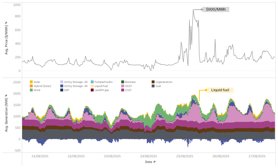
On 25 August 2025, Real-Time Market (RTM) prices reached the then market price cap of $900/MWh. A polar cold front held Perth to a maximum of 11.4°C, its coldest day in more than 50 years, and heating demand surged. At the same time, heavy cloud cover with sporadic breaks made rooftop solar generation volatile, leaving operational demand forecasts inconsistent and unstable.
The system turned to its usual answer: gas. But pipeline constraints curtailed OCGT output just when it was needed most, and liquid fuel units were brought on to cover the gap (Figure 1). Elevated daytime prices also discouraged Battery Energy Storage Systems (BESS) from charging, and their state of charge was less than 40% at the start of the ESROD period[1].
Figure 1: Average RTM price ($/MWh) and generation (MW) by technology, 21 to 27 August 2025
Source: Endgame analysis of AEMO WEM market data.
The event showed that the SWIS must withstand weather and fuel supply limits arriving together. Based on the supply conditions during the event, we estimate that gas for power generation was effectively limited to 406 TJ/day.
Repeated days like that, in a system with no coal left may bring system stress. So we asked the question: what happens to the transition if gas is constrained this way in the future?
Our reference case: SWIS Success
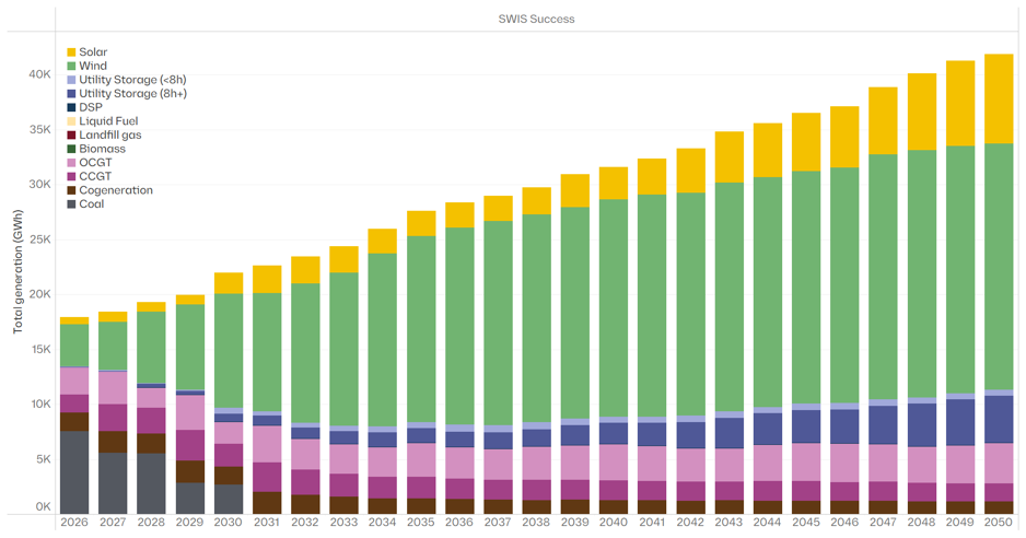
Our SWIS Success scenario describes a hopeful transition, supported by timely transmission and wind build-out. Figure 2 shows how generation changes over time. The system starts mostly with thermal plants, with coal supplying 42% of generation in CY 2026. By CY 2031, coal is retired and wind supplies most of the energy, with gas and storage firming. Solar generation slowly grows over time, peaking at 20% of generation in 2050.
Figure 2: Annual generation (GWh) by technology, SWIS Success, CY 2026 to CY 2050
Source: Endgame WEM price projection, Q3 2026.
Gas does a lot of work in this picture. In CY 2031, the first year without coal, gas-powered generation supplies around 36% of the system’s energy. Its share falls to about 20% by CY 2040, but it remains the firming resource.
Squeezing the gas
To test the daily fuel offtake constraint, we ran a Gas squeeze sensitivity on SWIS Success. Everything stays the same except for two changes. Gas available to generators is capped at 406 TJ/day, and plants can switch to liquid fuel if they have the functionality.
Over a year, 406 TJ/day is a lot of gas. The SWIS burns well under half of that for power in a typical year. So the constraint does not bite on annual volume. It bites on certain days, when demand is higher and renewable resources are lower.
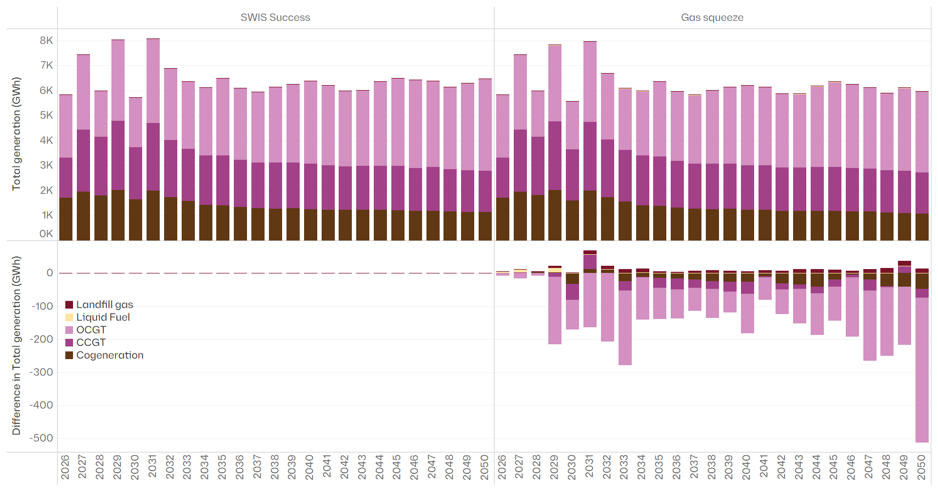
The bottom panel in Figure 3 shows how gas generation changes with the added constraint. Values below the line mean less gas generation in Gas Squeeze than in SWIS Success. From CY 2029, gas generation is lower in every year: by roughly 80 to 280 GWh a year through the 2030s and 2040s, and by more than 500 GWh in CY 2050. Most of that energy is replaced by solar and storage shifting across the day. Liquid fuel runs in CY 2026, 2027, 2029 and 2034, but never more than 13 GWh in a year.
Figure 3: Thermal generation (GWh) by technology, SWIS Success and Gas squeeze, and difference from SWIS Success
Source: Endgame WEM price projection, Q3 2026.
Small volumes, real price impact
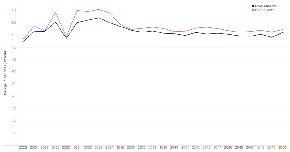
The squeeze raises average prices across the whole horizon (Figure 4). On constrained days, gas becomes scarce and more expensive resources then set the price more often; liquid fuel is called on in the tightest periods.
Figure 4: Average RTM price ($/MWh), SWIS Success and Gas squeeze, CY 2026 to CY 2050
CY 2029 to CY 2034. The squeeze adds $7 to $10/MWh (7% to 10%) in every year except CY 2030. This is the period when coal is retiring, and gas carries the most firming. Note that in 2030, CIS projects enter as renewable generation increases and prices drop.
CY 2037 onwards. Once new transmission projects enter, the renewable and storage fleet has matured, the increase settles at a persistent $2 to $6/MWh, averaging about $3.40/MWh.
The system copes, but it pays more to do so.
Resilience has a price
When gas is constrained, the system can’t firm renewables as well, and the SWIS has to rely on more expensive generation. Our Gas squeeze sensitivity tests one constraint, based on a real event. It does not yet test a worse renewable drought, a major outage or a more extreme weather event on top of that constraint.
As the SWIS becomes a weather-dependent system, knowing how it performs in bad conditions matters as much as knowing the central case. System planning exercises need more analysis similar to this, especially as the transition occurs.
Want to know more?
Our WEM price projection covers a range of scenarios and sensitivities. Subscribers receive the full report, a briefing, the assumptions and summary workbooks and half-hourly modelling results.
Results are from Endgame’s Q3 2026 WEM price projection (PLEXOS dispatch model). Prices are real, time-weighted average RTM prices in 2026 dollars. CY means Capacity Year: CY 2026 runs from 1 October 2026 to 30 September 2027.
Movement-driven charging demand and the limits of residential-anchored network planning – a Byron Bay case study
Endgame Analytics is pleased to share the third instalment of our decarbonising transport research series, this time turning to the light vehicle fleet and what happens when a large, mobile block of EV charging demand hits a network sized for locals, not visitors.
We modelled a Byron Bay case study, using Compass IoT connected vehicle data to size what an additional 6,000 visiting EVs would do to peak demand for the local substation. This reflects a peak visitor day, when around 40,000 visitors join 11,500 residents, and assumes half of visiting vehicles are electric. We also test how charger speed and tariff-driven charging behaviour change the result.
Some key highlights:
The peak roughly doubles on convenience charging alone: Against an 11.8 MW summer baseline, 6,000 EVs charging on arrival lift the peak to 23.9–25.1 MW, a 2.0–2.1x multiplier, regardless of charger speed.
Price signals could make it worse, not better: Time-of-use and solar-sharer tariffs synchronise the fleet to commence charging at the same time. On Level 2 (15 kW) chargers, peak demand rises to 91.9 -98.4 MW, 7.8–8.4x the 11.8 MW baseline, against about 25 MW for convenience charging.
Even perfect coordination doesn’t fully solve it: even the theoretical best case lifts the peak to 1.07x the baseline (12.6 MW) at 50% EV penetration, which would be 1.7x the baseline (19.5 MW) if EV penetration reaches 100%.
Pricing alone won’t coordinate this load. Direct load control, dynamic operating envelopes, and recognising the value drivers place on mobility will all need to be part of the answer, alongside the case for network augmentation itself.
Read the full paper here
Fill out the form to download the PDF
Get in Touch
Endgame Analytics are helping clients navigate these interactions between policy, technology, and economic strategy.
Martin Chow, Director (Endgame Analytics) | E: martin.chow@endgameanalytics.com.au
1. Confronting stochastic reality in the NEM to avoid planning blind spots
The way we plan the National Electricity Market (NEM) rests on a quiet assumption: that a handful of carefully chosen, deterministic input traces can stand in for a system that is, in reality, profoundly variable. Demand, weather, plant availability, gas use and price do not arrive as single, knowable numbers, they arrive as distributions. When we collapse those distributions to a central case and plan to it, we are not planning to reality. We are planning to an average the system may rarely, if ever, actually experience.
The danger is not that the central case is wrong. It is that everything around it, the tails, the compounding, the bad weeks, is precisely where reliability is won or lost, and a deterministic frame renders all of it invisible. This article makes three arguments:
That the inputs to our models are stochastic, so their outputs must be too.
That a system built to the average is not resilient to shocks without exposing itself to unserved energy.
That new tools, deliberate stress-testing and wargaming, backed by reform of the frameworks and the culture that commission them, can close these blind spots without throwing away what already works.
2. Modelling inputs are stochastic, and therefore outputs are stochastic too
Most modelling in the NEM is built on deterministic inputs. A planner selects a demand trace, a set of renewable traces, an outage assumption and a gas trajectory, runs the model, and reads off the result. It is clean and tractable, and it is not reflective of the system we actually operate. Demand, renewable output, forced outages, gas consumption, price and, ultimately, reliability are all stochastic. Each is better understood as a range of plausible outcomes than as a single line.
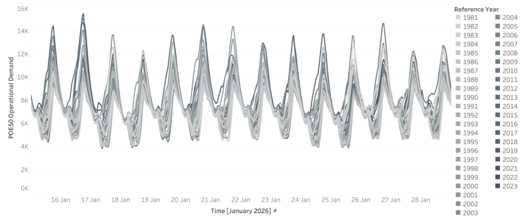
Start with demand. Figure 1 shows modelled NSW demand for a single fortnight, 15 to 28 January 2026, drawn across 45 weather reference years. The same calendar dates produce a wide envelope of outcomes depending only on which historical weather pattern is overlaid. A hot year sits well above a mild one, there is no single “January demand”, only a distribution of it.
Figure 1 – Demand in 2026 for NSW across 45 weather reference years (x-axis 15 January to 28 January, y-axis NSW demand)
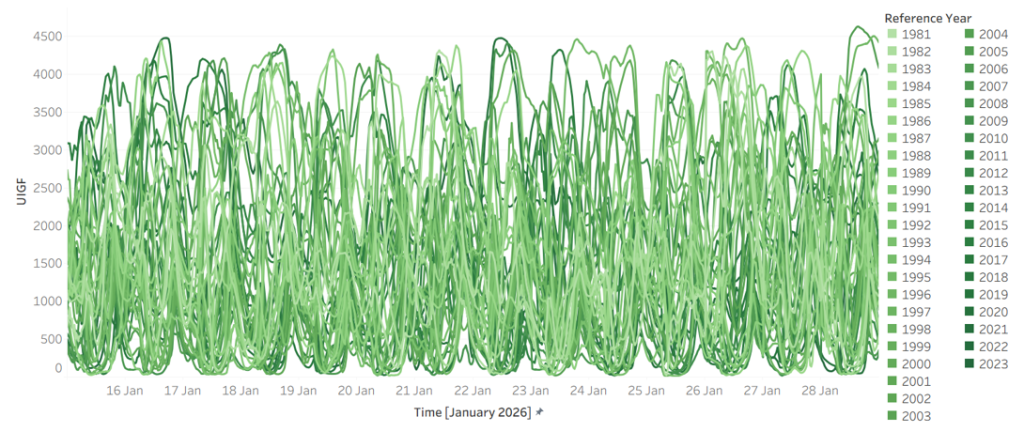
Weather is the driver, and it is at least as variable. Figure 2 shows Victorian wind generation over the same fortnight across the same 45 reference years. Output swings from near-zero to abundant over identical calendar dates, year to year. The combinations matter more than any single series: the years that deliver low wind are not always the years that deliver mild demand, and it is when high demand and low wind coincide that the system is most exposed.
Figure 2 – Wind in 2026 for Victoria across 45 weather reference years (x-axis 15 January to 28 January, y-axis VIC Wind)
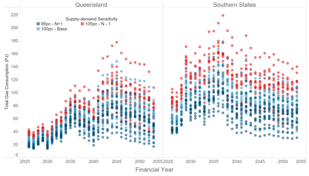
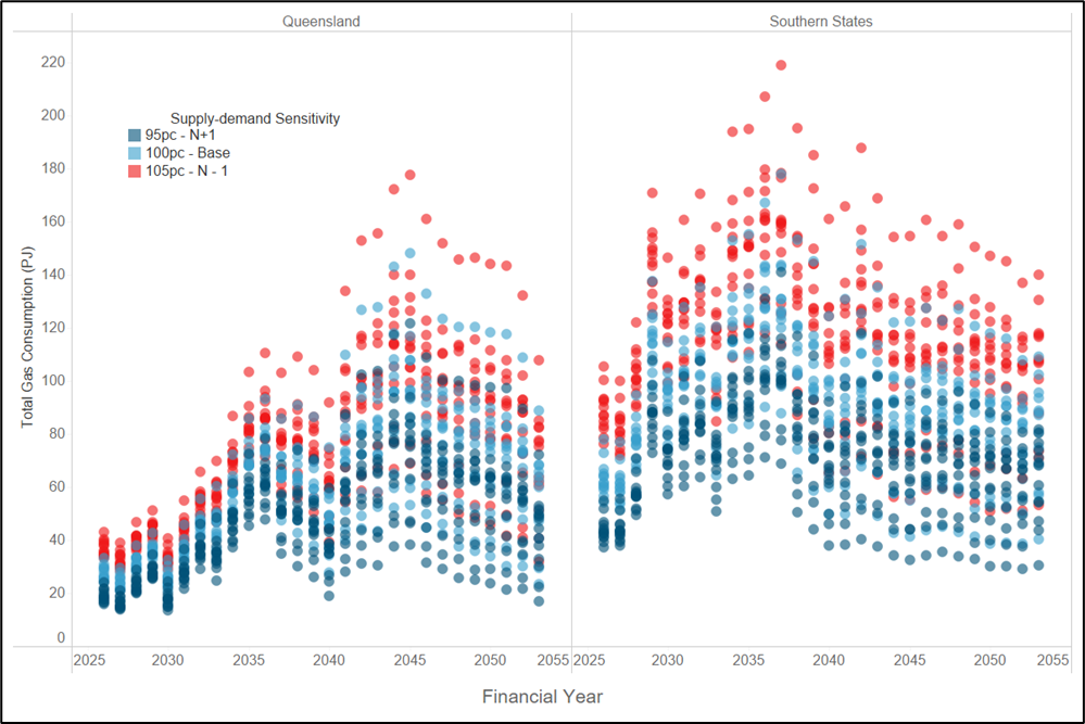
That variability propagates downstream. Figure 3 shows total gas consumption by gas-powered generation (GPG) by financial year, across reference years and under demand sensitivities of 95%, 100% and 105%. The spread is wide, and unsurprisingly so. GPG is the system’s reserve capacity, called on most heavily exactly when renewables are short and demand is high, so its consumption inherits and amplifies the variability sitting above it.
Figure 3 – Total gas consumption by GPG across reference years and supply sensitivities
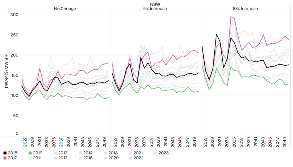
If the inputs are stochastic, the outputs cannot be anything else. Figure 4 makes this concrete: annual time-weighted average price (TWAP) in NSW under the Endgame Headwinds scenario, by weather reference year and under demand increases of 0%, 5% and 10%. A single deterministic run returns one number from this distribution, and, crucially, tells you nothing about how wide the distribution around it really is.
Figure 4 – Headwinds annual TWAP ($/MWh) in NSW by weather reference year and demand sensitivity
A deterministic model does not produce a wrong answer, it produces one draw from a distribution it never reveals. Two planners working from defensible but different central assumptions can arrive at materially different prices, dispatch patterns and reliability outcomes, with nothing in either result to signal how much sat unexamined in the tails.
3. A system built to the average is not resilient to shocks with unserved energy
The Integrated System Plan (ISP), the document that frames two decades of investment, uses a rolling reference year approach. It is a reasonable way to keep a twenty-year model tractable, but by construction it does not account for the stochastic nature of the NEM, and it tends toward a central, expected trajectory. That should prompt three uncomfortable questions. What does an average-based plan hide about how the system actually behaves? What does it tell us about the true shape of the operating envelope? And what does it tell us about resilience?
The honest answer to all three is: not enough. Averaging smooths away the very combinations that decide reliability, the simultaneous hot, low wind, high-outage conditions that seldom appear in a central case but routinely appear in the tails. A plan calibrated to the middle of the distribution can look entirely adequate while leaving no headroom for the adverse-but-plausible week.
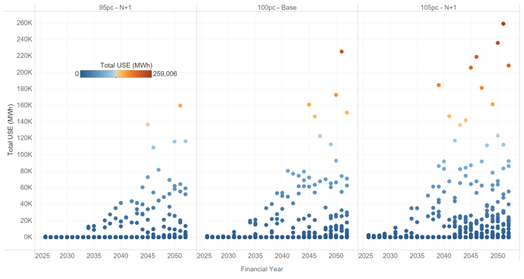
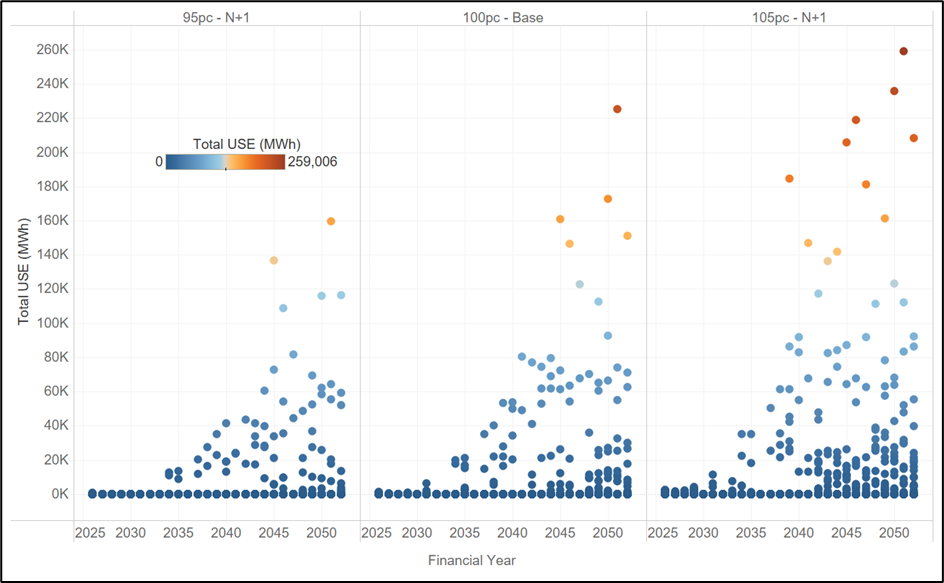
Figure 5 shows what surfaces when you look across the distribution rather than at its centre: projected unserved energy (USE) in NSW under the Endgame Sunny Side Up scenario, across 13 weather reference years and three demand sensitivities. In many years and sensitivities, USE is negligible. In others, it is not. A system that looks reliable on average can carry real unserved energy risk once the full spread of weather and demand it must withstand is accounted for, and that risk is invisible to any single central run.
Figure 5 – Projected USE in NSW for Sunny Side Up scenario across 13 weather reference years and 3 demand-supply sensitivities.
This is why “build to the average” is a dangerous frame. What keeps the lights on in a bad year is not the average outcome, it is the headroom the system carries against the tail. A plan that optimises to the centre will, almost by definition, treat that headroom as surplus and strip it out. The implication is uncomfortable but hard to avoid: the Electricity Statement of Opportunities (ESOO), in its current form, is no longer fit for purpose as a resilience instrument. A framework anchored to a narrow band of demand probabilities and weather years cannot characterise the risks that live in the tails, and those risks are exactly what we most need to understand.
4. New tools, wargaming and stress testing can greatly improve existing frameworks
None of this is an argument for discarding the ISP or the ESOO. The discipline they impose is real and worth keeping. We see the task in four parts: designing better studies, building the capability to run them, reforming the institutions that commission them, and breaking the culture that has held all three back.
The first shift is in how the studies themselves are designed. Too much is currently assumed away in the name of tractability. A more honest approach would:
Look much further into the future, to the system we are committing to deliver, not the system we have. The consequential question is whether the fleet we are spending billions to build will hold up under the weather and demand it will eventually face.
Characterise the full distribution of outcomes, moving beyond POE10 and POE50 demand traces and the handful of weather years that conventionally underpin reliability assessments, and drawing on much larger weather datasets.
Treat unit commitment and system security as part of the study, not an afterthought. Having enough energy on paper means little if the system cannot be operated securely when conditions are at their worst.
Bring gas demand and gas constraints inside the analysis. Gas-powered generation is the reserve capacity the system leans on in precisely the conditions that produce unserved energy, yet gas supply and transport limits are too often left at the edge of the model.
Deliberately try to “break” the system, actively hunting for the weaknesses and holes in the current approach, rather than assuming away the tough questions because they are inconvenient.
We can change our current planning frameworks using:
New tools. We need models that can be run faster, more cheaply and at far greater scale, so that exploring thousands of plausible futures becomes routine rather than exceptional. The combinatorics of weather, demand and outages cannot be brute forced with tools built for a handful of deterministic runs.
Wargaming. Borrowing from the security world, ‘blue team / red team’ exercises are a powerful device: one team is tasked with finding ways to break a future system, while the other works to remedy the weaknesses they expose. The adversarial structure uncovers failure modes that a single, consensus seeking study tends to overlook.
Stress testing. The aim is not only to ask whether a system is reliable, but to work out what it would take to break it. Knowing the distance to failure, and the conditions that get us there, is far more useful for decisions than a single pass/fail verdict against a central case.
5. Reforming the frameworks and the institutions
Better methods will not stick unless the regulatory framework asks for them, and two reforms stand out.
The first is to overhaul the ISP so that its centre of gravity shifts from transmission to the viability of the system as a whole. The process should assess future system needs and how the system will actually be operated, answering questions such as what the gas system will need to provide, what the system security requirements are, how the system will be operated through difficult periods, and what margin of safety is required to deliver adequate outcomes for society.
The second is to stand up an independent panel to stress test the system. A standing panel of industry experts should run stress testing and wargaming exercises on an annual basis. To keep them free from political interference, the exercises themselves should not be public, but the panel should publish a public facing report setting out its findings and recommendations. That structure preserves candour while keeping the conclusions accountable.
6. Breaking the groupthink
Underneath the technical and regulatory questions sits a cultural one. The current lack of innovation in how we model the future power system has produced a textbook case of groupthink: the same findings are confirmed again and again, and the ISP and ESOO processes are so heavily regulated that there is little room to do anything differently. The result is a planning conversation that mostly reinforces its own assumptions. Escaping it will take a governance structure that actively rewards new approaches rather than penalising those who depart from the consensus.
The NEM is becoming more weather dependent, not less. As thermal capacity retires and variable renewables and storage take its place, the gap between the average year and the bad year will only widen, and so will the cost of planning blind to it. The reasonable response is not to model the world as simpler than it is, but to confront its variability head-on: to treat stochastic inputs as stochastic, to plan for the distribution rather than its midpoint, and to build the margin of safety that resilience demands. This all starts with stochastic thinking.
Authored by: Kevin Yang, Matthew Bungate and Oliver Nunn
The road to net zero will need to include Australia’s freight task and the economics are shifting fast.
Endgame Analytics is pleased to share the second instalment of our decarbonising transport research series, this time focusing on road freight and the commercial viability of battery electric trucks (BETs) for long-haul operations.
We modelled a B-double trip between Brisbane and Sydney and found that BETs are closer to cost parity with diesel incumbents than conventional wisdom suggests.
Some key highlights:
Cost savings are real: Off-peak charging delivers a 6% cost reduction compared to diesel, while even peak charging brings the BET to within 1% of the diesel equivalent.
Distance matters: Cost parity is achieved at around 700 km per day under our baseline assumptions — and falls to under 300 km if diesel prices sustain above $3 per litre.
Capital is less of a barrier than you’d think: The unit cost per tonne-kilometre is relatively insensitive to the upfront price premium of the BET, as long travel distances amortise the higher acquisition cost effectively.
But structural barriers remain: Charging infrastructure gaps, fatigue regulation misalignment, and a fragmented operator market mean commercial viability alone won’t drive the transition. Coordinated government action is needed.
The convergence of the electricity and transport sectors creates a genuine opportunity. Operators who engage actively with energy market dynamics through strategic charging and vehicle-to-grid participation stand to benefit most.
Read the full paper here
Fill out the form to download the Electrification of Freight PDF
Get in Touch
Endgame Analytics are helping clients navigate these interactions between policy, technology, and economic strategy.
Martin Chow, Director (Endgame Analytics) | E: martin.chow@endgameanalytics.com.au
Isaac Mann, Consultant (Endgame Analytics) | E: isaac.mann@endgameanalytics.com.au
The electricity market will change how we drive. Is policy keeping up?
Endgame Analytics is launching a new research series on decarbonising transport. We are pleased to partner with SCT Consulting to explore the emerging electric vehicle market and its growing nexus with the electricity sector.
The shift to Battery Electric Vehicles creates a bi-directional relationship where charging behaviour affects grid stability, and electricity market volatility dictates transport costs.
Some key highlights:
Cost of Driving: BEV drivers will see fuel cost savings of between 65% to 100% compared to ICE vehicles, depending on when they charge — and with Vehicle-to-Grid technology, drivers could even be paid to charge.
Induced Demand: These lower operating costs have significant implications for future travel demand and congestion.
The Shadow Price of Mobility: Vehicle to grid technology introduces a new opportunity cost. Will drivers choose to forego a trip to capture the revenue from discharging to the grid?
Read the full paper here to understand the impacts on appraisal, policy, and the future research needed to support the transition.
Spot prices are the mechanism by which the energy market signals the needs of the power system to participants, investors, and consumers. So when we see something strange occurring in the behaviour of spot prices, it warrants attention. In this article we examine how spot prices are becoming more ‘noisy’ (ie, they are oscillating more frequently). We present analysis of spot price noise, some preliminary theories about what is causing it, and what the consequences may be.
What do we mean by noise?
First, we must define the concept of spot price noise. From a mathematical perspective, noise is the transient oscillation of a time series that is typically overlaid on top of some underlying trend. Note however that ‘noise’ is typically random, although it is not entirely without structure.
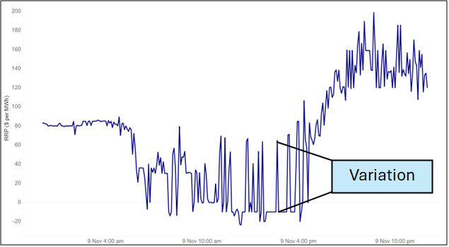
For our purposes, we use the mathematical concept of ‘variation’ as our proxy for noise – ie, the difference between any two consecutive intervals between the spot prices. For example, when spot prices for 4 intervals are $50, $100, $75, $20 then the variation outcomes are $50, -$25, -$55. Figure 1 illustrates the concept of variation on a recent day for NSW.
Figure 1 – Illustration of variation; NSW 9 November 2025
Given that we are not interested in scarcity events where prices signal underlying shortage of generation, we have capped all prices at $300 per MWh before calculating variation. We do not see these outcomes as noise, but rather an important signal in prices to reflect scarcity. In addition, when summing variation over time we will also use the concept of the absolute value of variation to capture both positive and negative movements, which might otherwise cancel each other out.
Variation has been rising
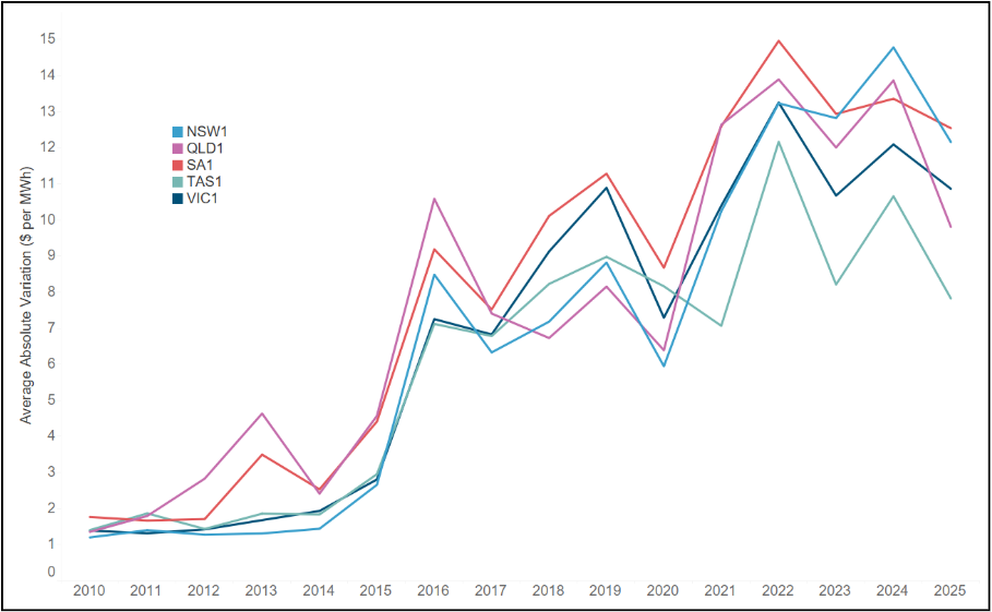
What has been happening to variation over the history of the NEM? Figure 2 shows the average absolute variation from 2010 to 2025 for each region of the NEM. The rise in variation is enormous. In 2010, the average difference between 2 dispatch intervals was around $1 per MWh across all regions; in 2025 that number exceeded $10 per MWh.
Figure 2 – Average absolute variation by NEM region, 2010 to 2025
What else do we know about variation?
Figure 3 shows average variation by time of day for NSW in 2010 and 2025. Two observations:
Variation has increased across the day, but it is greater at some times than others. This would be expected due to the presence of the duck curve, but there are also increases in variation during the middle of the day and overnight.
There appears to be a periodicity to the average variation in 2025 – it exhibits spikes that seem to occur with a regular frequency.
Figure 3 – Average variation in NSW by time of day, 2010 versus 2025
It is this second feature that is of most interest. Why should there be any intraday structure to the average noise if it is indeed just caused by random perturbations in the supply and demand curves? Is there something causing the noise that means it is in fact partially deterministic rather than purely stochastic?
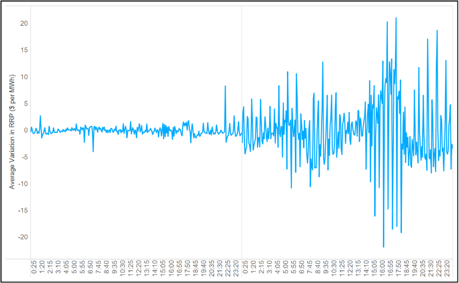
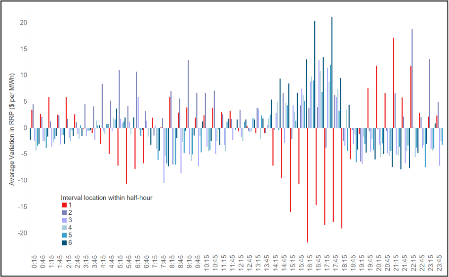
Figure 4 shows the average variation by time of day for NSW. To aid in the visualisation we have added colours to each observation based on where the dispatch interval occurs during the half-hour (ie, a number between 1 and 6).
Figure 4 – Average variation in NSW by time of day, Calendar Year 2025
The results are striking:
The positive spikes in variation tend to occur in the last 5 minutes of the half hour (shown in dark blue).
The negative spikes in variation tend to occur in the first 5 minutes of the half-hour (shown in red).
There is a clear structure to the variation depending on the location within the half-hour.
This seems to suggest that the ‘noise’ we are seeing is, at least in part, being driven by something structural that depends on the temporal location within the half-hour.
Why is variation so structured?
With 5-minute settlement having been in effect for some time, the temporal structure of variation is surprising – why does it matter whether it is the first or last interval of the half-hour? There are only two possible overarching causes: demand or supply. We start with a look at supply.
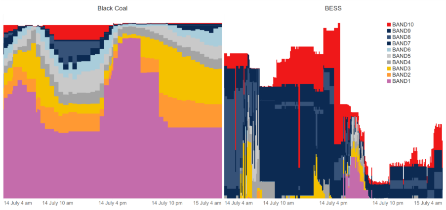
A simple analysis of bids in NSW reveals at least one possible reason for the structure. Figure 5 shows a recent sample of the aggregate final bid stacks for NSW Black coal on the left and NSW BESS on the right. Interestingly, the bid stack of NSW Black Coal is defined on a half-hourly basis, whereas BESS varies by 5-minute interval.
Figure 5 – Sample of bids for NSW black coal and NSW BESS
This would suggest that the supply curve is flat within the half-hour. We have analysed the bids for all thermal generators in the NEM, and a large proportion of them still supply bids on a half-hourly basis. Interestingly, Snowy’s bids are defined on a 5-minute interval basis.
Much more analysis would be required to pin down the exact relationship between noise and the supply-demand balance. But at this stage, we posit that an increased variability in both demand and VRE have led to increased variability in the exact point at which supply clears against demand. At the same time, bid structures have remained relatively lumpy and have not (with the exception of batteries and some hydro) adapted to the changing conditions. The root cause of the change in noise warrants deeper analysis, but the 30-minute structure of bids seems a good starting point.
What are the consequences of the increase, and possible vanishing, of noise?
Noise is a big part of the battery business case. Noise lifts the highest daily prices and drops the lowest daily prices. This increases the opportunity for arbitrage by batteries. Indeed, the challenge of obtaining a high ‘percentage-of-perfect’ outcome is driven by the increased presence of noise, which makes it harder to time charging and discharging to achieve an optimal outcome.
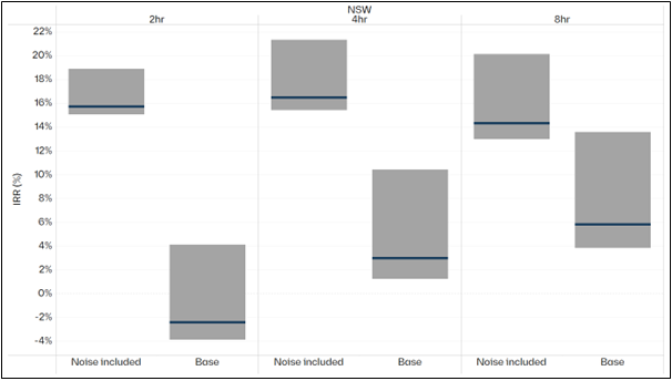
Figure 6 shows the range of returns to batteries in NSW of different durations with and without historical levels of noise being included in the modelling.
Figure 6 – IRR for indicative battery of different durations in NSW, noise versus base
The shorter the duration of the battery, the more dependent it is on noise. This makes sense because as duration increases, the spread of each full cycle must capture higher buy points and lower sell points.
Were noise to increase, the relative business case for shorter duration batteries would improve. Alternatively, were noise to decrease, the business case for shorter duration batteries would be more adversely affected than for longer durations.
It follows that investors and market participants need to have a better understanding of how the inclusion of noise affects their projects, and to stress-test their models to include different levels of noise.
Finally, we note that it is unclear whether noise is a feature or bug of the NEM. In particular, is it:
a sophisticated signal provided by the energy only market, that we do not yet understand; or
a pathological outcome of bidding behaviour that is making it harder to invest and make sensible decisions.
More to come from us on this in the coming months.
Late last year we published a piece examining the importance of weather and stochastic variables to price outcomes. Since then, we have repeatedly been asked to explain how these stochastic variables behave, their influence on price outcomes, and the broader implications for the grid. We have been uplifting our own capabilities in modelling these stochastic factors. Most notably, we are increasingly conscious of the implications of there being a wide range of possible outcomes for reliability. Against this backdrop, in this article, we examine how outcomes differ when we alter weather and demand-supply (i.e., assumptions about adding or losing a major unit). We show that an analysis of median or average outcomes based on a single weather reference year, and a single set of demand assumptions is wholly inadequate for understanding variability, uncertainty and risk, and most importantly the reliability of the system. We want to stress test the system that is implied by a median set of conditions and see how it performs.
Moving from averages to distributions
The computational complexity of running market models means that it is costly in terms of time and computational resources to run many different simulations of the future. Average or ‘typical’ conditions are used as the basis for most long-term capacity expansion forecasts for this reason. Yet this is no longer enough. We cannot shoehorn a stochastic system into a deterministic model – we are misleading ourselves if we think that this will be adequate to guide us through the maze of complexity that awaits us in a high penetration renewable future.
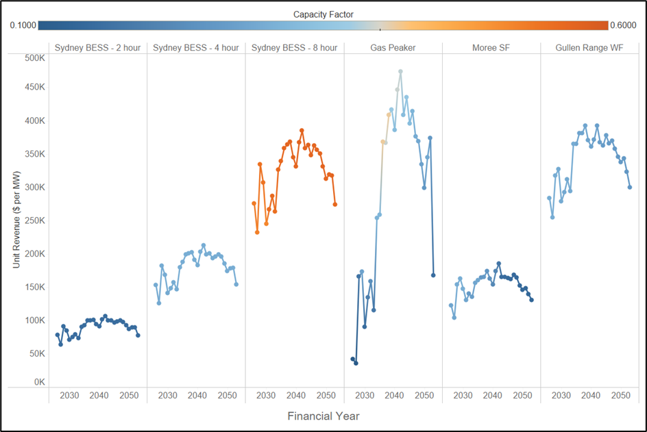
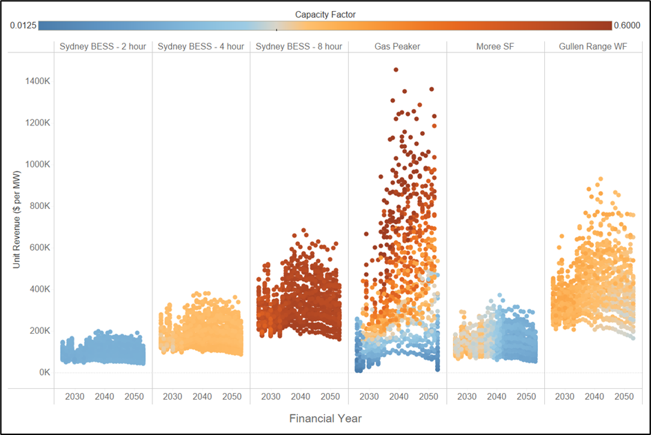
Figure 1 shows the average revenue per megawatt for a range of assets in NSW under a median weather reference year, and a single realisation of demand. For the purposes of this article, we have used Endgame’s Sunny-side up scenario as the basis for our forecasts. This scenario assumes a new build profile that is based on a median weather reference year, with a high (POE10) assumption about demand. The colour scale shows the capacity factor of each of the assets. We note the following:
Longer duration batteries make more money per MW of installed capacity.
Gas proves its value later in the horizon, as renewable penetration increases.
Wind makes solid returns because our modelling assumes constraints on the new build of this technology, limiting new entry from competing away profits.
Figure 1 – Revenue per MW for a single weather year for assets in NSW
But how does this picture change when we consider many different reference years and allow for ups and downs in supply (eg, N-1 or N+1 relative to forecast). The result is shown in Figure 2. Each dot represents a single realisation of revenue per megawatt for a single year.
Figure 2 – Distribution of revenue per MW for 3 demand sensitivities, 13 weather years
We observe the following:
The upside for longer duration batteries is far greater than for shorter duration batteries.
The range of outcomes for wind is far greater than for solar.
The most striking outcome is that gas generation can earn super-normal profits in some years, and in other years it can fail to earn anything.
What does this mean for the gas supply system?
The differences between the outcomes in Figure 1 and Figure 2 completely changes how we should think about each of these assets, and the system as a whole. For example, consider the implications for gas consumption via gas-powered generation (GPG). Figure 3 shows the differences in total GPG consumption across each weather year and demand sensitivity. We can see differences in a given year of up to 120 PJ across the southern states.
Figure 3 – Distribution of GPG for 3 electricity demand sensitivities, 13 weather years
This gives rise to many questions, such as the following:
What does this mean for planning purposes?
What is the value of ‘insurance-style’ assets that can deliver gas in outlier years?
How resilient is our current system to these types of events?
How do we reward gas production and transportation and long duration pumped hydro facilities that may only be required with a low probability?
What does this mean for gas turbines that are contracting for gas supply?
Indeed, the consequences are too many to enumerate here. But the key point is that unless we understand the distribution of outcomes, we have no chance of planning for the future that awaits us.
Stress testing to understand reliability
We have examined the consequences for gas, but what does this mean for system reliability? Our analysis shows that the variability of output for renewables has consequences for the reliance on gas. But what about unserved energy (USE) – ie, how often will weather and demand variability lead us to run short of generation, and how far are we at any point in time from shedding load?
Figure 4 below shows the consequences for unserved energy across 13 weather reference years and 3 demand-supply sensitivities. The result is that as renewable penetration increases over time, although the median conditions exhibit no USE, the distribution has long tails.
As the system becomes more stochastic, the importance of considering these extreme events only grows. By the 2040s we are in a situation where a shock to the system leads to outcomes that would not be considered reasonable by consumers (eg, 50-100 times the reliability standard in NSW). We note that these are driven by plausible and quantifiable variations in supply and demand, rather than ‘black swan’ events that may be examined by others in the sector.
Figure 4 – Projected USE in NSW for Sunny-side up scenario implied by distribution across 13 weather reference years and 3 demand-supply sensitivities.
This is not intended to be taken a criticism of renewables, but rather an observation that current modelling of single realisations of the future is inadequate to inform the needs of the system. We need a different approach. We make the following recommendations:
We need to start stress testing the system of the future, and understanding how variability in weather, demand, and gas supply influence reliability and resilience. In our opinion, the current ESOO is a solid starting point, but does not address the question of how we should go about filling the gaps that it identifies.
We need to think about how the assets that will provide resilience to these events will be rewarded in the market. Even with a very high market price cap, a generator that is only required under very extreme circumstances may never get built because of the challenges of obtaining financing for assets that are only used in 1 in 50 or 1 in 100 year events.
Finally, stress testing needs to consider all elements of the energy supply chain. From gas supply to hydrology and network availability. Models that can provide insights into these risks will help us build a system that exploits the many advantages of renewables, but recognises and addresses the blind spots of a high VRE system.
In conclusion, we need to understand that the nature of risk in this future system is fundamentally different to that which existed in our legacy system, and that our existing approaches may give highly misleading answers as to reliability and risk.
We have seen solar and batteries at the core of government schemes over the last year, and indeed further back in time. In addition, the Commonwealth has sought to make the most of solar resources by encouraging consumption during the middle of the day with its Solar Sharer Offer. And finally with the challenges facing the roll-out of wind, gas and pumped hydro projects, we are left in a world where many of our clients have said to us that solar is the only option for investment. Against this backdrop, we ask the question how hungry is our current market for solar, and what can we learn about the returns that solar will earn from the energy only market?
Average prices in 2025
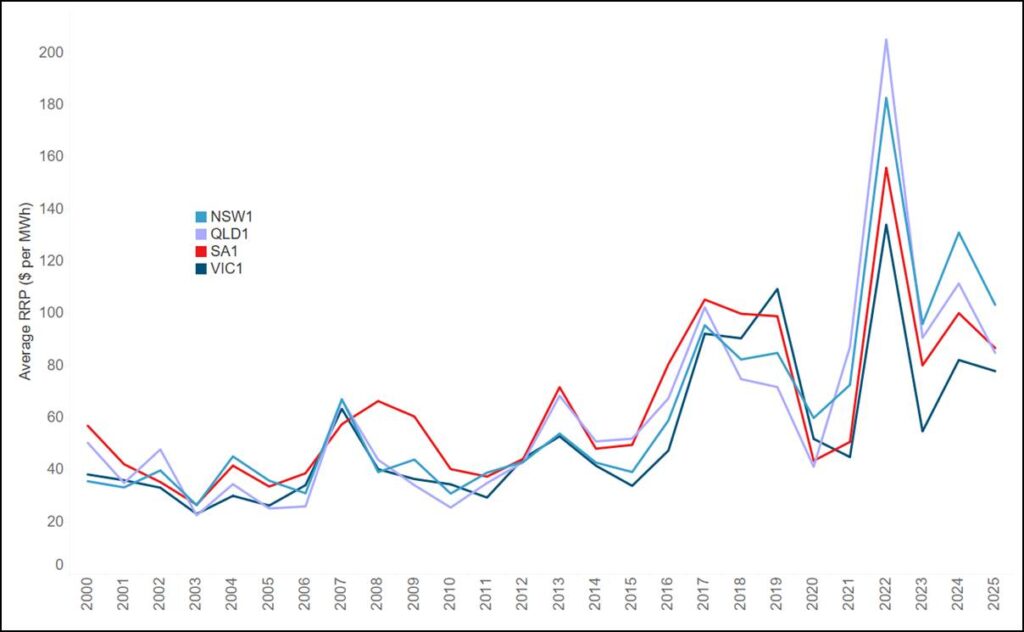
As a starting point, we examine historical average prices for the mainland regions of the National Electricity Market (NEM). Figure 1 shows that 2025 prices were lower in all regions than 2024 prices but have risen from their levels in 2023. New South Wales experienced the highest average price of $103 per MWh, with Victoria the lowest at $77.9 per MWh.
Figure 1 – Average calendar year prices for mainland regions of the NEM, 2000-2025
Average prices for different periods of the day
Average prices are a good starting point to understand the returns to solar, but the marked feature of prices over the last decade has been the deepening duck curve.
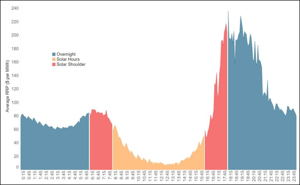
Figure 2 shows the average dispatch price by time of day for Victoria in 2025. We have coloured the different times of day according to solar output during these periods, namely:
Solar hours, which are 8 am to 4 pm.
Solar shoulder hours, which are 6 am to 8 am and 4 pm to 6 pm.
Overnight periods, from 6 pm to 6 am.
The belly of the duck (ie, the solar hours) is markedly lower than the shoulder and overnight periods, as has been seen for some time.
Figure 2 – 2025 average Victoria prices by time of day, coloured by solar definition
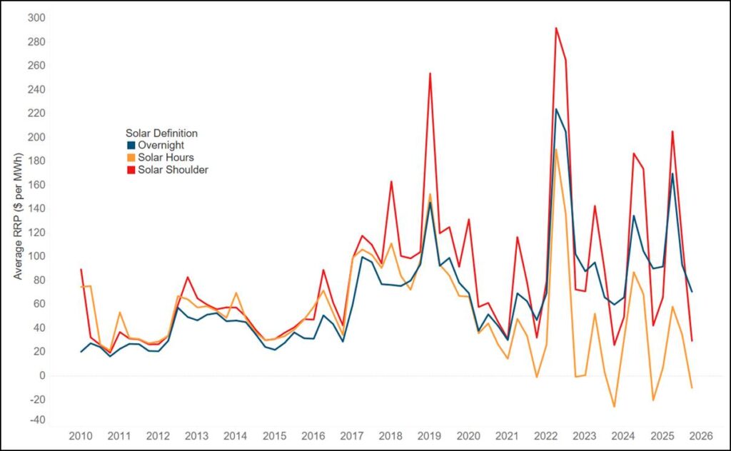
An immediate question is how prices for each of these time periods have changed over time with the increasing penetration of solar. Figure 3 shows the Victoria quarterly average price for each of the three categories: solar hours, solar shoulder, and overnight.
We note the following:
Over the period from 2010 to 2020, overnight and solar periods experienced very similar outcomes, but from 2021 onwards there has been a marked divergence between solar and overnight periods.
Prices for solar hours have collapsed in recent years and have now often become negative on average for entire quarters, namely Q4 2023, Q4 2024 and Q4 2025.
There is a clear quarterly pattern emerging with the highest prices in Q2 and Q3.
Figure 3 – Victoria quarterly average prices by solar category, 2010 to 2025
Bringing revenue into the equation
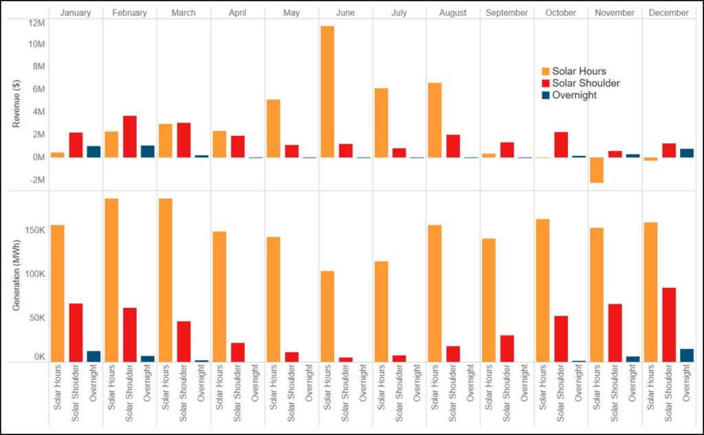
Average price is a very helpful indicator of the available pie for solar, but if we want to look more deeply at returns it is necessary to incorporate dispatch volumes, which vary greatly over the course of the year. With that in mind, Figure 4 shows the monthly revenue and generation by solar category for all solar farms in Victoria for 2025.
We note the following:
38 per cent of all revenue is earned in the solar shoulder, with the remainder coming from solar hours.
Counterintuitively, the vast majority (ie, 90 per cent) of revenue from solar periods is earned winter when output from solar is at its lowest. Indeed, revenue from solar periods was negative during Q4.
The relationship between generation and revenue is not straightforward – more generation does not necessarily lead to more revenue, because when we generate during the year matters.
Figure 4 – Revenue and generation across all solar units in Victoria by solar category
Looking to the future – solar earns the bulk of its revenue in winter
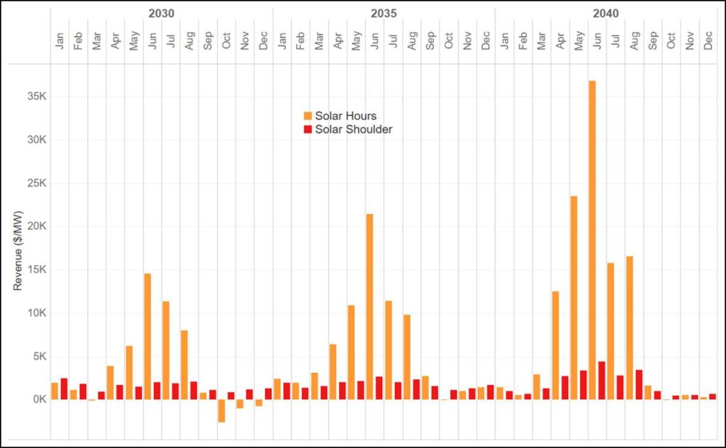
We can also project forward to see how the system will evolve using one of our house scenarios, ie, Endgame’s Sunny Side Up Scenario. Figure 5 shows average Victoria revenue per MW for three financial years by month and solar category for this case. We project that the pattern of the increasing significance of winter continues – indeed, by 2039-40 our modelling shows that solar will earn virtually nothing from September to March save for the small amount of output during the solar shoulders. In addition, the relative importance of the shoulder decreases from around 30 per cent of revenue to 16.5 per cent by FY2040.
Figure 5 – Projected Victoria solar revenue per MW; FY2030, FY2035, FY2040
What does this mean?
Solar revenues in summer have collapsed. Solar must now justify itself through contribution to the system during winter, particularly when the system is becalmed, ie, when wind output is low. Even with the large amounts of batteries that are projected to enter the system, this outcome does not change. The success of solar, and particularly rooftop solar, has led to a world where the system will be awash with energy in summer and so the marginal value of the technology is greatest when its output is relatively low.
We conclude with the following observations:
Solar earns most of its money when it is operating at a relatively low proportion of nameplate capacity. It follows that any curtailment which occurs during summer may be largely irrelevant to the overall revenue of a site.
Financiers need to be comfortable that they are buying an asset that makes most of its money when it is generating well beneath its capacity. Our own modelling shows that large proportions of solar revenue may come from periods where it is generating at less than 30 per cent of nameplate.
The massively seasonal nature of solar revenue makes a strong case for seasonal storage of any form of energy. Technologies that can move megawatt-hours between seasons will be extremely valuable in this context.
Given the large amount of variability in the occurrence and frequency of wind droughts from one year to the next, it follows that solar spot revenue will be incredible volatile. This is borne out by our own analysis of outcomes for different weather reference years. Batteries cannot mitigate this risk – deeper forms of energy storage and gas are required to hedge load.
The challenges of building gas and wind have left many in the industry turning to a combination of solar and batteries as the answer to the transition. But what is the relative cost of building enough solar and storage capacity to meet power requirements 24 hours a day, 365 days a year, for a reasonable set of conceivable weather years? And how much more does it cost than including wind and gas in the generation mix? Against this backdrop, in this article, we ask: what is the long-run marginal cost of supplying a flat load for various allowable sets of technologies?
The concept of Long Run Marginal Cost
Marginal cost refers to the additional expense incurred to produce one extra unit of output. Marginal cost is a critical concept in microeconomics and economic regulation. Importantly:
Marginal costs look to the future, not to the past: it is only future costs for which additional production can be causally responsible; it is only future costs that can be saved if that production is not undertaken.
-Alfred Kahn
There are both short run and long run notions of marginal cost. The distinction is whether all factors of production are fixed or can be varied, ie:
the short run marginal cost is the cost incurred to produce one extra unit of output, holding at least one factor of production constant; and
the long run marginal cost is the cost to produce one extra unit of output assuming all factors of production can be varied.
We will focus on long run marginal cost (hereafter ‘LRMC’). There are many ways to estimate LRMC, but for the purposes of this discussion we will use a standalone or greenfields method. This roughly assumes the cost to rebuild the whole system from scratch. LRMC is therefore equal to the average system cost were we to rebuild the whole system from nothing.
The key word to consider here is average. The art of estimating LRMC lies in what we average over. Do we consider a single day, a single month, a single weather reference year? Or do we average over all possible outcomes? The challenge is that there can be significant differences between the costs of supplying a megawatt-hour of energy depending on when that megawatt-hour is consumed.
For the purposes of this discussion, we consider a broad possible set of megawatt-hours, ie, how much it costs to supply one megawatt hour, when that megawatt-hour could have been consumed in any of the last 13 years. This is effectively saying that the cost of building a resilient system is the cost to supply energy under any weather conditions that have prevailed in recent memory.
LRMC versus levelised cost of electricity
It is critical to understand the difference between LRMC and the levelised cost of electricity (LCOE). Before the advent of renewables, LCOE was a helpful way of comparing technologies like coal and gas, whose output closely matched the profile of demand. But when the profile of generation from technologies varies greatly over time – as is the case with renewables – this simplistic measure ceases to be relevant. Indeed, LCOE provides highly misleading estimates of cost because it does not capture the time-dependent nature of generation costs, ie, that there are some times of the day or year that are significantly harder to supply.
Consider the profile of a solar plant. This profile is drastically different to the profile of system demand, wind output, or simply a flat load. LCOE is the average cost of generation, not the average cost of supplying load. It tells us the cost of generating some profile of output, not the cost of meeting demand. This is a critical difference, because it means that LCOE is now of virtually no benefit in understanding the costs that consumers face.
So what is the LRMC of a unit of energy?
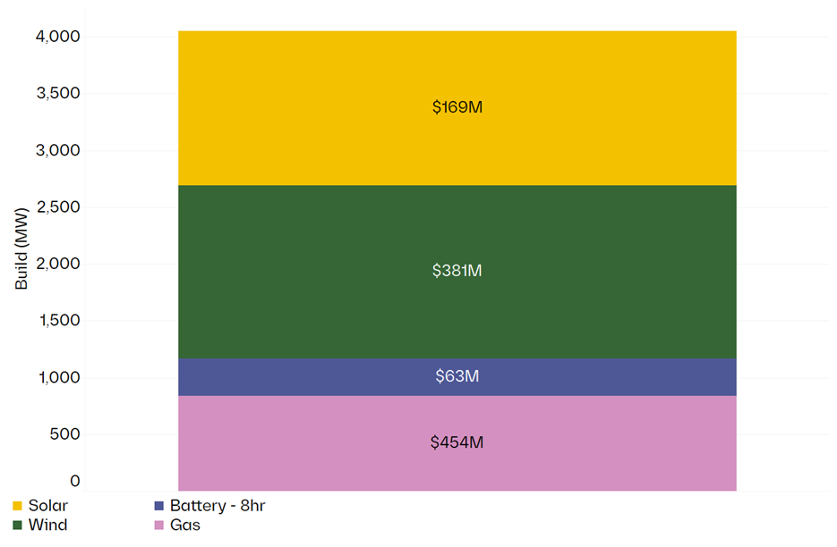
We start by considering the LRMC when all technologies are available. For explanatory purposes, we have calculated the LRMC on the basis of supplying 1 GW of flat load. Figure 1 below shows the generation mix that our optimisation model yields: 1.5 GW of wind, 1.3 GW of solar, 0.3 GW of 8-hour batteries, and 0.8 GW of gas. The total cost – and so the LRMC – of the generation is $122/MWh (the sum of the system costs shown on the graph, dividing by the load served over the year).
Figure 1 – 4 GW of capacity are required to meet 1 GW of load at least cost
Optimal generation mix to supply 1 GW of flat load, NSW, median weather year
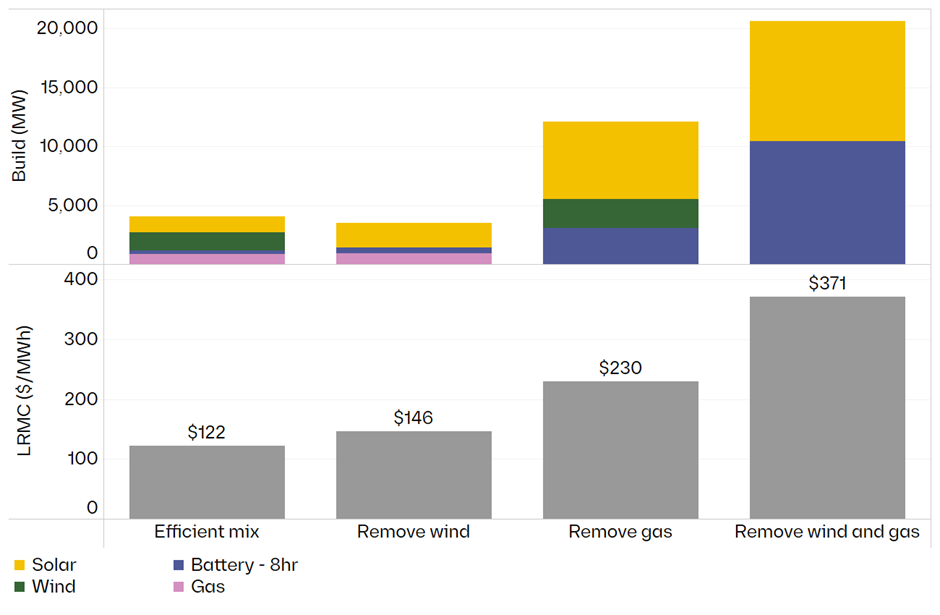
But what if we limit the set of allowable technologies. Figure 2 shows the generation mix and the change in cost (on a dollars per megawatt-hour basis) from removing wind, gas, and both wind and gas from the system.
Figure 2 – As we remove technologies from the mix, LRMC rises massively
Optimal generation mix to supply 1 GW of flat load and related sensitivities, NSW, median weather year; attendant LRMC shown in bottom panel
We note the following:
In the absence of wind, the LRMC rises from $122 per MWh to $146 per MWh.
If we remove gas from the equation, the LRMC rises from $122 per MWh to $230 per MWh.
A system that relies solely on solar and batteries will have a cost of $371 per MWh, ie, $3.2 billion for a single year.
What happens when we change the weather reference year?
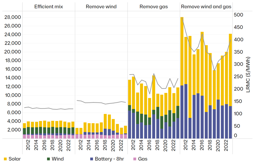
An important input assumption is the weather reference year, ie, the assumed temperature, wind and solar irradiance profiles that underpin the modelling. Figure 3 shows the same analysis as Figure 2, but for 13 weather reference years. The difference between the median and the extreme outcomes can be substantial and speaks to the resilience of the system.
Figure 3 – The cost of a new system depends on the assumed weather
Optimal generation mix to supply 1 GW of flat load for 13 reference years versus attendant LRMC, NSW.
What does this mean?
I draw four conclusions from this analysis:
First, running a reliable, high penetration renewable system without gas is virtually impossible. If we really believe in the need for renewables, we must work out a solution for the supply of gas and gas-powered generation as well.
Second, in the absence of wind, the cost of the system is substantially higher, particularly when we consider the outcomes across different weather years. If we want to reduce costs for consumers, we need to work out a way of getting wind into the system, and that will require not just investment in wind but also transmission.
Third, building a system that is resilient to all weather conditions will be markedly more expensive than one that is reliable ‘on average’, unless we have access to all available technologies.
Finally, even in the world where we consider all possible technologies, the LRMC is markedly higher than many of projections that we see across the market. We need to level with consumers that wholesale prices will have to be higher than historical levels to make investments whole.
The narrative that we can complete the transition with solar and batteries, ensure a reliable system, and keep prices low is fundamentally at odds with the facts. Instead, we need to focus on unlocking constraints on technologies that can limit price increases and building a resilient system that can ensure reliable supply not just on average but at the extremes. If we continue to perpetuate the myth that solar and batteries can do everything, we will be left with a brittle, unreliable, and expensive system that does not meet consumers’ needs. Ultimately, this will hinder rather than help the transition.