1. Confronting stochastic reality in the NEM to avoid planning blind spots
The way we plan the National Electricity Market (NEM) rests on a quiet assumption: that a handful of carefully chosen, deterministic input traces can stand in for a system that is, in reality, profoundly variable. Demand, weather, plant availability, gas use and price do not arrive as single, knowable numbers, they arrive as distributions. When we collapse those distributions to a central case and plan to it, we are not planning to reality. We are planning to an average the system may rarely, if ever, actually experience.
The danger is not that the central case is wrong. It is that everything around it, the tails, the compounding, the bad weeks, is precisely where reliability is won or lost, and a deterministic frame renders all of it invisible. This article makes three arguments:
- That the inputs to our models are stochastic, so their outputs must be too.
- That a system built to the average is not resilient to shocks without exposing itself to unserved energy.
- That new tools, deliberate stress-testing and wargaming, backed by reform of the frameworks and the culture that commission them, can close these blind spots without throwing away what already works.
2. Modelling inputs are stochastic, and therefore outputs are stochastic too
Most modelling in the NEM is built on deterministic inputs. A planner selects a demand trace, a set of renewable traces, an outage assumption and a gas trajectory, runs the model, and reads off the result. It is clean and tractable, and it is not reflective of the system we actually operate. Demand, renewable output, forced outages, gas consumption, price and, ultimately, reliability are all stochastic. Each is better understood as a range of plausible outcomes than as a single line.
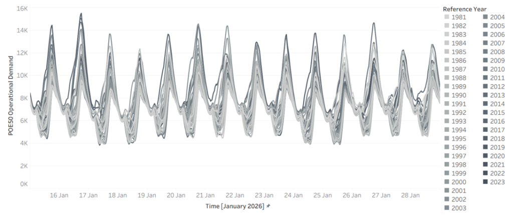
Start with demand. Figure 1 shows modelled NSW demand for a single fortnight, 15 to 28 January 2026, drawn across 45 weather reference years. The same calendar dates produce a wide envelope of outcomes depending only on which historical weather pattern is overlaid. A hot year sits well above a mild one, there is no single “January demand”, only a distribution of it.
Figure 1 – Demand in 2026 for NSW across 45 weather reference years (x-axis 15 January to 28 January, y-axis NSW demand)
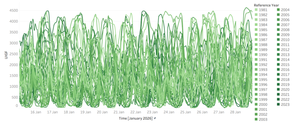
Weather is the driver, and it is at least as variable. Figure 2 shows Victorian wind generation over the same fortnight across the same 45 reference years. Output swings from near-zero to abundant over identical calendar dates, year to year. The combinations matter more than any single series: the years that deliver low wind are not always the years that deliver mild demand, and it is when high demand and low wind coincide that the system is most exposed.
Figure 2 – Wind in 2026 for Victoria across 45 weather reference years (x-axis 15 January to 28 January, y-axis VIC Wind)
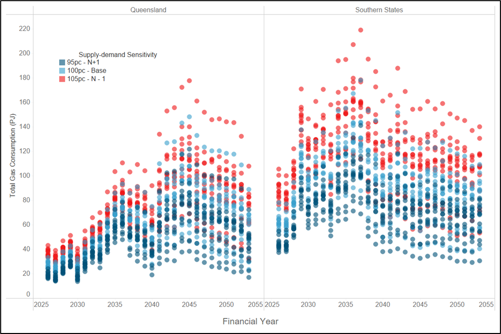
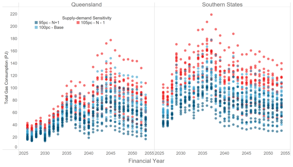
That variability propagates downstream. Figure 3 shows total gas consumption by gas-powered generation (GPG) by financial year, across reference years and under demand sensitivities of 95%, 100% and 105%. The spread is wide, and unsurprisingly so. GPG is the system’s reserve capacity, called on most heavily exactly when renewables are short and demand is high, so its consumption inherits and amplifies the variability sitting above it.
Figure 3 – Total gas consumption by GPG across reference years and supply sensitivities
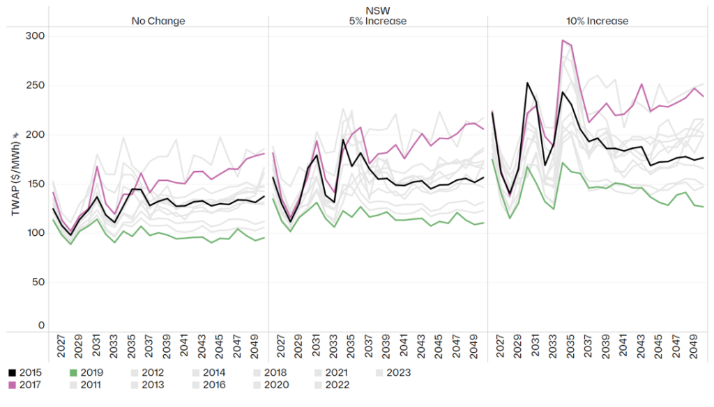
If the inputs are stochastic, the outputs cannot be anything else. Figure 4 makes this concrete: annual time-weighted average price (TWAP) in NSW under the Endgame Headwinds scenario, by weather reference year and under demand increases of 0%, 5% and 10%. A single deterministic run returns one number from this distribution, and, crucially, tells you nothing about how wide the distribution around it really is.
Figure 4 – Headwinds annual TWAP ($/MWh) in NSW by weather reference year and demand sensitivity
A deterministic model does not produce a wrong answer, it produces one draw from a distribution it never reveals. Two planners working from defensible but different central assumptions can arrive at materially different prices, dispatch patterns and reliability outcomes, with nothing in either result to signal how much sat unexamined in the tails.
3. A system built to the average is not resilient to shocks with unserved energy
The Integrated System Plan (ISP), the document that frames two decades of investment, uses a rolling reference year approach. It is a reasonable way to keep a twenty-year model tractable, but by construction it does not account for the stochastic nature of the NEM, and it tends toward a central, expected trajectory. That should prompt three uncomfortable questions. What does an average-based plan hide about how the system actually behaves? What does it tell us about the true shape of the operating envelope? And what does it tell us about resilience?
The honest answer to all three is: not enough. Averaging smooths away the very combinations that decide reliability, the simultaneous hot, low wind, high-outage conditions that seldom appear in a central case but routinely appear in the tails. A plan calibrated to the middle of the distribution can look entirely adequate while leaving no headroom for the adverse-but-plausible week.
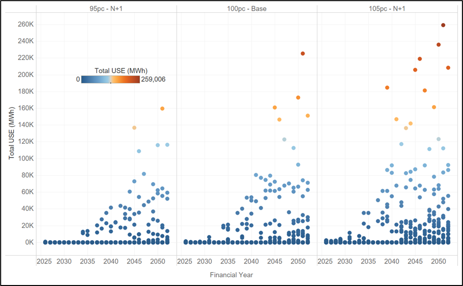
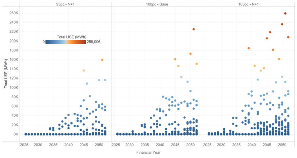
Figure 5 shows what surfaces when you look across the distribution rather than at its centre: projected unserved energy (USE) in NSW under the Endgame Sunny Side Up scenario, across 13 weather reference years and three demand sensitivities. In many years and sensitivities, USE is negligible. In others, it is not. A system that looks reliable on average can carry real unserved energy risk once the full spread of weather and demand it must withstand is accounted for, and that risk is invisible to any single central run.
Figure 5 – Projected USE in NSW for Sunny Side Up scenario across 13 weather reference years and 3 demand-supply sensitivities.
This is why “build to the average” is a dangerous frame. What keeps the lights on in a bad year is not the average outcome, it is the headroom the system carries against the tail. A plan that optimises to the centre will, almost by definition, treat that headroom as surplus and strip it out. The implication is uncomfortable but hard to avoid: the Electricity Statement of Opportunities (ESOO), in its current form, is no longer fit for purpose as a resilience instrument. A framework anchored to a narrow band of demand probabilities and weather years cannot characterise the risks that live in the tails, and those risks are exactly what we most need to understand.
4. New tools, wargaming and stress testing can greatly improve existing frameworks
None of this is an argument for discarding the ISP or the ESOO. The discipline they impose is real and worth keeping. We see the task in four parts: designing better studies, building the capability to run them, reforming the institutions that commission them, and breaking the culture that has held all three back.
The first shift is in how the studies themselves are designed. Too much is currently assumed away in the name of tractability. A more honest approach would:
- Look much further into the future, to the system we are committing to deliver, not the system we have. The consequential question is whether the fleet we are spending billions to build will hold up under the weather and demand it will eventually face.
- Characterise the full distribution of outcomes, moving beyond POE10 and POE50 demand traces and the handful of weather years that conventionally underpin reliability assessments, and drawing on much larger weather datasets.
- Treat unit commitment and system security as part of the study, not an afterthought. Having enough energy on paper means little if the system cannot be operated securely when conditions are at their worst.
- Bring gas demand and gas constraints inside the analysis. Gas-powered generation is the reserve capacity the system leans on in precisely the conditions that produce unserved energy, yet gas supply and transport limits are too often left at the edge of the model.
- Deliberately try to “break” the system, actively hunting for the weaknesses and holes in the current approach, rather than assuming away the tough questions because they are inconvenient.
We can change our current planning frameworks using:
- New tools. We need models that can be run faster, more cheaply and at far greater scale, so that exploring thousands of plausible futures becomes routine rather than exceptional. The combinatorics of weather, demand and outages cannot be brute forced with tools built for a handful of deterministic runs.
- Wargaming. Borrowing from the security world, ‘blue team / red team’ exercises are a powerful device: one team is tasked with finding ways to break a future system, while the other works to remedy the weaknesses they expose. The adversarial structure uncovers failure modes that a single, consensus seeking study tends to overlook.
- Stress testing. The aim is not only to ask whether a system is reliable, but to work out what it would take to break it. Knowing the distance to failure, and the conditions that get us there, is far more useful for decisions than a single pass/fail verdict against a central case.
5. Reforming the frameworks and the institutions
Better methods will not stick unless the regulatory framework asks for them, and two reforms stand out.
The first is to overhaul the ISP so that its centre of gravity shifts from transmission to the viability of the system as a whole. The process should assess future system needs and how the system will actually be operated, answering questions such as what the gas system will need to provide, what the system security requirements are, how the system will be operated through difficult periods, and what margin of safety is required to deliver adequate outcomes for society.
The second is to stand up an independent panel to stress test the system. A standing panel of industry experts should run stress testing and wargaming exercises on an annual basis. To keep them free from political interference, the exercises themselves should not be public, but the panel should publish a public facing report setting out its findings and recommendations. That structure preserves candour while keeping the conclusions accountable.
6. Breaking the groupthink
Underneath the technical and regulatory questions sits a cultural one. The current lack of innovation in how we model the future power system has produced a textbook case of groupthink: the same findings are confirmed again and again, and the ISP and ESOO processes are so heavily regulated that there is little room to do anything differently. The result is a planning conversation that mostly reinforces its own assumptions. Escaping it will take a governance structure that actively rewards new approaches rather than penalising those who depart from the consensus.
The NEM is becoming more weather dependent, not less. As thermal capacity retires and variable renewables and storage take its place, the gap between the average year and the bad year will only widen, and so will the cost of planning blind to it. The reasonable response is not to model the world as simpler than it is, but to confront its variability head-on: to treat stochastic inputs as stochastic, to plan for the distribution rather than its midpoint, and to build the margin of safety that resilience demands. This all starts with stochastic thinking.
Authored by: Kevin Yang, Matthew Bungate and Oliver Nunn