A beginner’s guide to wholesale market modelling
Context – where we left off
Last time we completed our description of the end-to-end modelling process. But we noted that there remained many different tricks and tips that were hidden from the layperson.
With that in mind, we promised that in our final instalment in the series we would examine the assumptions and methods that fall into the category of ‘the Dark Arts’ of modelling.
At the outset, we make clear that our intention is to shed light on these often overlooked parts of the modelling process. We want the reader to understand what models can and cannot do, and the ways, means, and devices that together are sometimes used that can make it hard to derive value from modelling exercises. We want to arm you with the basics of ‘Defence against the Dark Arts’.
In the remainder of this article, we explain our thoughts on the top four ‘Dark Arts’ of the modelling process, specifically:
- Crude chronologies – playing with time itself.
- Carbon budgets and renewable targets – hiding costs in shadow prices.
- Market based new entry – a no longer necessary evil.
- Post-processing of results – what is helpful and what is not.
We conclude by setting out how we think about the role of modelling, and the philosophy that underpins our own work in this area.
Crude chronologies – playing with time itself
For capacity expansion, it is necessary to simplify the number of periods (sometimes called time slices or load blocks) over which we model the system. For example, a single day might be represented by 3 time slices: one for each eight-hour period of the day. In turn, this day might represent 30 days, which have similar characteristics. In so doing, 30 * 24 =720 hours could be represented by a mere 3 time slices.
The benefit is that the problem is easier, and so faster, to solve. But the approach of using very few time slices has been limited by the advent of:
- intermittent renewables, whose output shapes change greatly from one day to the next over the course of the year, and
- storage devices that force us to use time slices that obey a time-sequential chronology (ie, a set of time slices where time constraints are preserved).
It is now the case that unless we use a very large number of time slices, the system that results from the capacity expansion problem is not resilient. The solution is to use more time slices – this is not really an option, unless we are looking at a very simple power system.
Despite this reality, some modellers often want to speed up the process, or do not have access to commercial solvers, and so they resort to use of a crude set of time slices. The outcome can often be a brittle or, on the other hand, massively overbuilt system. When working with a consultant using capacity expansion modelling, it is worth being aware about the assumptions they have made as to time slices – a Dark Art if ever there was one.
Carbon budgets and renewable targets – hiding costs in shadow prices
One of the powerful aspects of using an optimisation framework for solving models is the ability to impose constraints. It is trivial to add constraints to the model that do the following:
- Place a limit on the amount of CO2 emissions that can be produced in a given timeframe.
- Force in a particular level of renewable generation by some date.
- Represent other limits or restrictions on the operation of the capacity expansion model.
In practice, these constraints are just like any other constraint, such as the supply-demand constraint, or a limit on the amount of generation that can connect in a region. These constraints have the potential to change the outcomes that would have otherwise occurred in their absence.
When these constraints are imposed, the model will do whatever it takes (such as over-building renewable or artificially suppressing thermal generation out-of-the-merit-order) to meet these targets. This will occur regardless of whether the new investment will recover its costs from the energy prices in a potentially over-supplied market. This is not a fault of the least cost expansion model per se – imposing these constraints is to assume they will be met regardless of the cost, and the model is faithfully satisfying the request of the modeller by identifying the cheapest way to meet these requirements.
However, a modeller should know to look for these ‘hidden costs’. Just like the supply-demand constraint, every constraint in the model gives rise to a ‘shadow price’. As explained in our first article, this is the marginal value of alleviating this constraint by one unit on the total system cost. In the case of a renewable target or carbon budget, there is a clear meaning to their associated shadow prices:
- In the case of a carbon budget, it is the implied cost of abatement of (the last) tonne of CO2 – ie, the implicit cost of reducing CO2 emissions due to the additional clean technology investment required.
- In the case of a renewable target, it is the implied subsidy per MWh that is required to achieve that level of renewable penetration. This could be seen as the renewable energy certificate value that is required to make renewables whole.
Of incredible importance is that, when we invoke these constraints, the prices that fall out of the capacity expansion model assume that there is also a carbon emissions price, and a renewable energy certificate price. And so if we look only at the price that falls out of the model and assume this will be the cost of electricity, we will fail to account for the effect of the assumed carbon and renewable energy certificate prices, or the ‘missing money’ that must be funded outside the wholesale electricity market. These ‘hidden’ prices are often overlooked or forgotten about, but they are critical to understanding how generation recovers its costs. Moreover:
- without some sort of carbon price or emissions trading mechanism, it makes no sense to include a carbon budget constraint; and
- without some sort of subsidy to renewables, it makes no sense to include a renewable energy target constraint.
It is critical to be aware of this – otherwise we are not going to factor in the whole cost of policies, and so we may not understand what is required to achieve them.
Market-based new entry – a no-longer necessary evil
One of the perennial questions in the sector is whether a least-cost capacity expansion model is the correct way to determine new entry. The alternative, which is used by many advisors, is called ‘market-based new entry’.
The recent surge of market-based new entry
Recent years have seen a surge of market-based new entry in market modelling. We often hear the motivation of using this approach is that new entrant generation built by least-cost capacity expansion models does not seem to earn enough pool revenue to recover its costs. Market-based new entry appears to fix this problem by allowing the modeller to alter the investment path manually until the all new entrants recover their costs.
We will address the economic fallacy of market-based new entry shortly. However, it is first worth noting that in a market where renewables are built to meet ambitious government renewable constraints or carbon budgets, new entrants will not recover their cost from pool prices alone. This is because of the “missing money” phenomenon discussed in the last section. The least cost expansion model merely exposes this fact, which is either misunderstood or ignored by proponents of market based new entry when communicating their results.
The quasi-economic argument against least-cost capacity expansion
One argument against least-cost new entry is that the decision to build is based on cost rather than price which is what we see in the market. The argument is quasi-economics at its best. It fails to recognise that price is inherently linked to long run marginal cost, and so solving for cost gives us the outcome we seek.
The proponents of market-based new entry fail to recognise that the capacity expansion model solves for cost but also produces prices. These prices are equal to the long-run marginal cost of generation. Taken to its logical conclusion, a market-based new entry proponent would suggest that dispatch also needs to be ‘based on price’. This would involve iterating between different combinations of plant to be dispatched in a given interval until eventually we stumbled upon the same outcome that is yielded by the dispatch engine. Why would we do such a thing, when we can get the answer directly by solving as a linear program?
Market based new entry as a low-quality capacity expansion model
In the absence of constraints, the prices yielded by the least-cost capacity expansion are exactly the level needed so that every technology recovers its costs. In effect this is equivalent to a world where investors build new plant right up until the point where any additional plant would be uneconomic. This is also the common goal shared with market-based new entry.
Put another way, we see the following outcomes:
- Least-cost capacity expansion satisfies the requirement that every plant that gets built receives a price that at least satisfies the costs over the life of the plant. At its best, market based new entry should do the same, but this is not guaranteed by the iterative process.
- Least-cost capacity expansion satisfies the requirement that whenever price is high enough to support a new entrant, it gets built. Again, at its best, market based new entry should do the same, but this is not guaranteed by the iterative process.
The key phrase here is ‘at its best’. In reality, the market-based new entry process is trying to solve a very complicated problem with very primitive mathematical machinery. We know that some consultants complete this process manually, with choices being made by an analyst on-the-fly. This is essentially ‘dealer’s choice’ – ie, the outcomes depend on the gut-instinct of the modeller.
Even when an algorithm, or heuristics, are codified in a program, there is no guarantee that the process will converge to an outcome that satisfies both (a) and (b) above. The chances of stumbling on the exact combination of build over the next 25 years that yields prices that walk the tightrope between (a) and (b) above is vanishingly small. This means that there will always be either plants that are not built that should have been, or plants that are built that should not have been.
The computational argument against least-cost capacity expansion
A decade ago, least-cost capacity expansion models took a very long time to solve, and so required very crude chronologies. These models therefore were internally consistent but gave a poor representation of the planning needs of the system. It was not uncommon for these models to lack resilience. Against this backdrop, market-based new entry was an alternative but sometimes necessary evil to provide a meaningful view of the future needs of the power system.
However, in the last decade the speed of solvers has improved dramatically. Gurobi can now solve a least-cost capacity expansion problem with thousands of time slices per year over a 25-year horizon in a matter of hours. It is no longer necessary to stumble around with iteration and primitive heuristics to find a profile of the needs of the system. What was once a helpful tool to plan out the system is now no longer necessary, and there is no basis for it.
Market-based new entry is now a Dark Art
As the system becomes increasingly complex, market-based new entry becomes less and less helpful for planning, resilience testing, and projections of the future needs of the system. For example, when we have been asked to reconcile market-based new entry models against the results of least-cost capacity expansion, we find that there are either large amounts of unserved energy, or many plants that are built that do not recover their costs.
More importantly, the ‘dealer’s choice’ phenomenon means that we cannot easily replicate or reproduce the analysis of other consultants who have used market-based new entry. Outcomes based on choices made in the early hours of the morning by a bleary-eyed analyst as to what plant should get built where, are not consistent with robust modelling practices.
The continued use of these models without recognition of their limitations is surely one of the most prevalent Dark Arts of the sector.
Post-processing of results – what is helpful and what is not
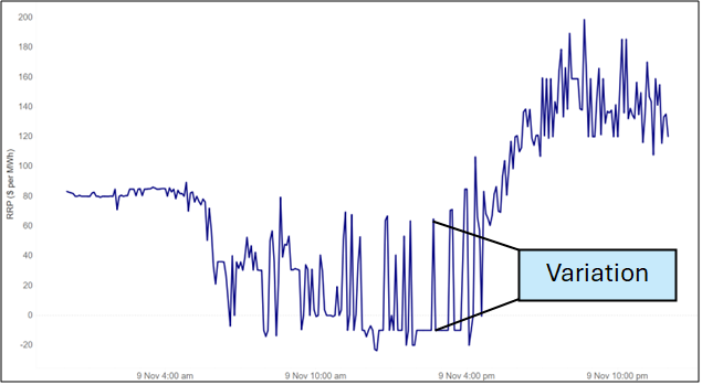
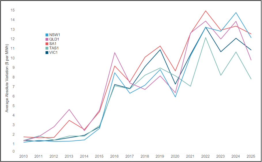
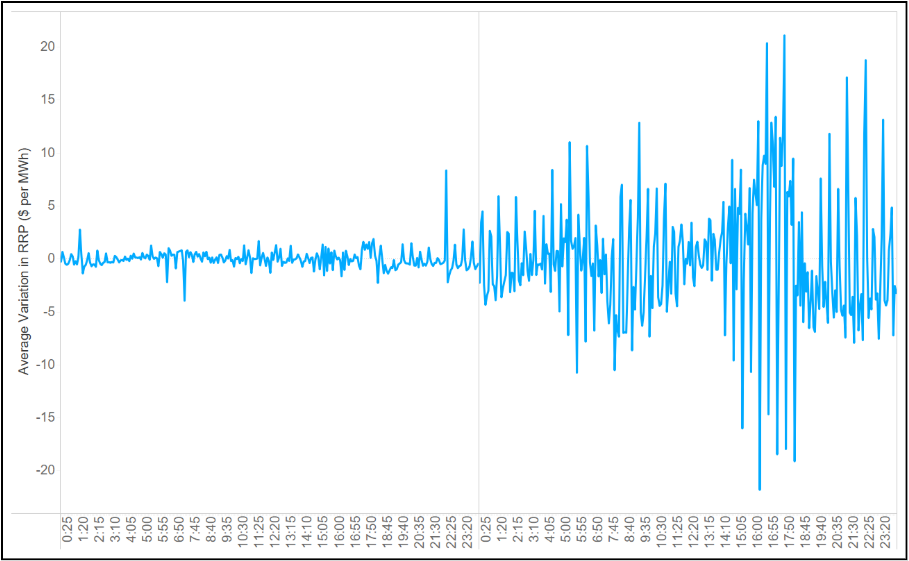
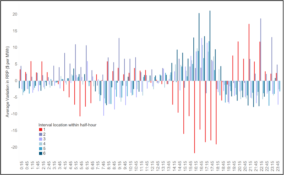
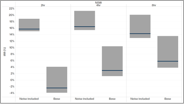
By now it has become clear that there are elements of the market and the power system that are fundamentally challenging to capture. And so not everything can be included in the capacity expansion and operational dispatch models. Many consultants (ourselves included) provide services that alter the outputs of the model in a post-processing step. For example, it is not unusual to add interval-to-interval volatility or ‘noise’ to prices to reflect the patterns we see in the market.
We do not see anything wrong with this, provided it is clear as to what is the effect of this post-processing. Advisors should decompose their results so that the contribution of these post-processing steps can be captured – sometimes they are highly material to their findings.
In addition, some post-processing seeks to account for high-impact system events (such as the Callide C explosion) that cannot be meaningfully included in a small number of deterministic model runs. This is not to say that models cannot simulate this type of price impact if we know exactly when and how they happen in the future. In fact, the revenue impact on other assets, which is what most commercial clients are interested in, can even be easily obtained via back-of-the-envelope calculations. The real challenge is to project the frequency with which such events will happen and how the system unfolds immediately following it, which is often highly event-specific and beyond the realm of market simulation models. Including events of this type in a projection of the future and pretending that there is a sophisticated methodology for ‘modelling’ them goes beyond the Dark Arts and verges on the Unforgivable Curses. Market models are not designed to simulate such events – be wary of anyone telling you they can do so.
Conclusion – what’s it all about
We have listed here some of the Dark Arts, but in truth there are too many to list. Modellers can always use sleights of hand, and tricks to deceive their audience – the Dark Arts. In my opinion, the problem here stems from our understanding of the purpose of modelling. From my perspective, the purpose of a model is to create a mental latticework on which we can build intuition. When constructed properly, that latticework will remain rigid and so will not simply yield to your gut instincts – it will require that you adhere to its assumptions and logic, and so build your own understanding of the problem. We can change the latticework (through changing assumptions) but that gives rise to a new set of constraints on our logic.
In contrast, when we force models to yield to our own intuition, and to give us the answers that we want, those models lose all meaning. This is why modelling is particularly unhelpful in adversarial processes, where the objective is to show that one model is ‘wrong’ and one is ‘right’. Models were never meant to be ‘wrong’ or ‘right’ – they were meant to inform our thinking.
Sometimes models give us helpful insights, and sometimes they do not. But once problems become sufficiently complex, without them we are left without any sound basis for decision making. The energy industry poses many such problems, where the stakes are high, and the risks are many. We are foolish to leave decision-making to gut instinct alone and not use models, but the more we can learn about those models and understand them, the better our decisions will be. A more informed world is the outcome. Our purpose in discussing this topic is to arm you with the basics of ‘Defence against the dark arts’. This is the information you need to understand both what models cannot do, but more importantly the many powerful questions that can indeed be answered by modelling if we are able to stretch our understanding.
